Loops that Matter is method for finding out which links and feedback loops are responsible for generating observed model behavior. The theory behind the approach is described in a paper by Schoenberg, Davidsen and Eberlein. That theory is used to animate diagrams during simulation, list the feedback loops important to driving behavior, and allow the generation of simplified causal loop diagrams to highlight key feedback loops.
Loops that Matter is built into the Stella Software and is available at all times for your use as you develop and analyze models. It will be activated on any existing models you have developed that are not too large, though you can also choose to turn it on for larger models.
With the release of Version 2.1 of the software we have updated the computation of link scores for flows to be based on the change in the flow relative to the change in the net flow, instead of the flow relative to the net flow. This formulation has the advantage of being independent of flow formulations since it does not matter whether values are added in a flow equation, or two separate flows are created.
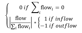
In the original LTM formulation the link score from a flow to a stock was given by
This formulation has a weakness in that a flow that is constant can be weighted more strongly than a flow that depends on other variables and this distorts the value of the loop scores passing through the flow. Since all the other link scores are based on changes in auxiliary (converter) values, we revised the link scores for flows to have this same property:
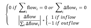
This formulation emphasizes the change in the flow caused by changes in other model variables which is a more robust measure. It can be shown that this formulation is independent of the exact formulation of flow values used.
You can change whether Loops that matter is active from the Model Settings Properties Panel. Simply check or uncheck the  checkbox. By default this will be checked for new models, and for small models created in previous versions. If it is not checked, no loop dominance information will be computed or displayed.
The heart of Loops that Matter is the link score which, simply put, is the contribution of one model variable to the change in another model variable. Link scores are computed for connectors, and also for flows. The polarity of the link score corresponds to the polarity of links in a causal loop diagram. A positive value means that a change in the source variable will cause the target to change in the same direction (or for flows that the source is an inflow) while a negative value means that the target will change in the opposite direction (or for flows that the source is an outflow). When you simulate a model with LTM turned on, you will see an animation using link scores:
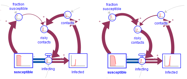
This shows the animated Link Scores before and after the peak of infections. The animations are based on the relative link scores, so the thickness shows how important one input is relative to another. In the example above, you can see that the link from "contacts" to "risky contacts" is important at first, and that later the link from "fraction susceptible" to "contacts" becomes important.
Red links are reinforcing (R/+). Blue links are balancing (B/-). Gray links are inactive. (Steel gray links are of unknown polarity (U).
To see the value of the link scores over the course of the simulation, open the results panel and click on the arrowhead of the link. For flows out of a stock click on the flow right next to the stock the flow is coming out of (the arrowhead if it is a biflow). The results panel will display the relative contribution of the link over the course of the simulation.
The absolute value of the relative link scores will always add to one, which means that the thickness of the arrows coming in will always add to (roughly) the thickest arrow. This means you can, for example, have a thin and thick arrow, or two medium arrows.
There is a builtin called PATHSCORE that allows you to record the Loop Scores computed between two or more variables (along a path the link scores are multiplied as described below). This number is not relative to other link scores, and can be very large in magnitude, especially when a model approaches equilibrium. See Specialized builtins for details on usage.
An important characteristic of Link Scores is that they can be multiplied together along a path and maintain the interpretation of the impact of the starting variable on the ultimate target. When that target is the variable itself, as it will be for a feedback loop, the score along that path, created my multiplying all of the Link Scores. is called the Loop Score. Just as Link Scores can become quite large, Loop Scores can become quite larger. However, at any point in time it is possible to normalize the Loop Scores by making them add up to 100%. This normalized Loop Score tells us how important the loop is in determining behavior at a point in time.
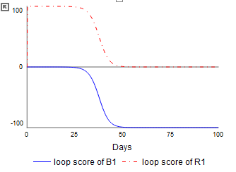
Loop Scores change over the course of the simulation. In the simple bass diffusion example above there are two loops, and their scores are:
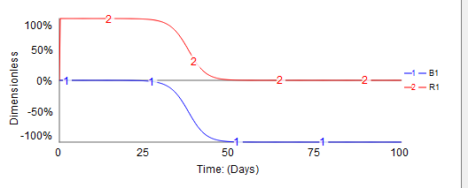
This information is available in the Loops Panel. The reinforcing loop starts out explaining 100% of the behavior (looks like exponential growth), then there is a transition in which the balancing loop starts to gain importance till it explains 100% of the behavior. We use the sign of the loop to distinguish balancing and reinforcing loops so the value is displayed using negative numbers in the graph.
It is also possible to create variables that capture loop scores.
These variables are created from the Loops Panel, and use the LOOPSCORE builtin. Unlike other built in functions, the loop scores are only available after the simulation has been completed. So the output of the variables while the model is running will always be NAN.
Once the feedback loops in a model have been identified and scored, it is possible to create causal loop diagrams that only show the variables and loops critical to generating observed behavior. Some of the theory behind this is described in a paper by Schoenberg, but in a nutshell it is possible to filter out variables and loops to only show the most important ones:
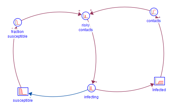
In this particular example, both loops are important, but the extra variables have been filtered out. The CLD presented is controlled from the Loops Panel.
In more complicated models, there may be a number of loops that are partially overlapping in the variables they include and have similar effects on behavior. While the impact of the individual loops will be correct, the contribution of any one of them may be small. If, in a model with 20 loops, there is one set of 5 that have similar contributions to behavior over the course of the simulation, it can be convenient to consider all 5 together. If those 5 loops together explain 50% of the behavior, and there are another 4 that are similar to one another explaining 30% of the behavior, then a simplified 2 loop explanation of 80% of model behavior may be possible.
To enable consolidation of similar loops, LTM computes the correlation between the different loops identified. This correlation can then be used to group together like loops that are similar. By specifying a correlation cutoff, LTM will aggregate like loops together based on the correlation, and the inclusion of overlapping structure (two loops must share a link to be combined in this way). This can reduce the total number of loops.
While what correlation cutoffs are best is a subject of ongoing research, current experience suggests that setting a cutoff of 80% using relative loop scores or of 95% and using the raw loop scores to do the correlation yields the best reduction in complexity without discarding important differences. For any individual model, experimentation with cutoff values may yield more insights. If the model oscillates or approaches equilibrium many raw loop scores may be highly correlated as they pass through near infinity points. The correlation cutoff can be set in the Loops Panel.
Canceling loops are a very similar concept - effectively these are negatively correlated loops. They often occur because of the exact nature of formulation used in a model. For example if a variable has an equation a-b+... where a and b are bother driven by the same variable you might end up with a positive loop through a and negative through b, but together they simply cancel their effect on d - so it is sensible to ignore both loops. This cancellation is done automatically by LTM, but can be turned off in the Loops Panel.
When analyzing behavior there are differences in how much is changing at any point in time. For example, with a damped oscillator there is significant change when the oscillations are big, and this diminishes to effectively 0 when the model reaches steady state. The triggering mechanism for the change might be external, for example a step input, or it might be internal as in the case of shifting loop dominance.
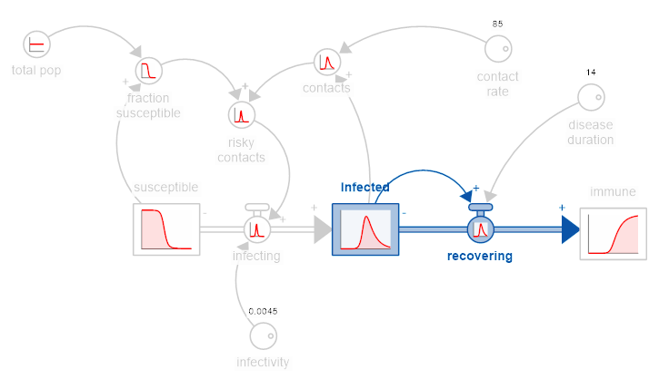
Consider for example, a simple SIR model:
If we look at the contribution of the different loops we have:
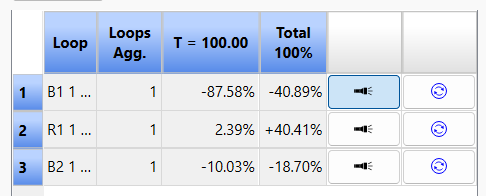
Loop B1 - which is highlighted above - is dominant over the course of the simulation. But it is most important only after loops R1 and B2 have moved the system from largely susceptible to largely infected or recovered. If we look at the two flows over the course of the simulation they show:
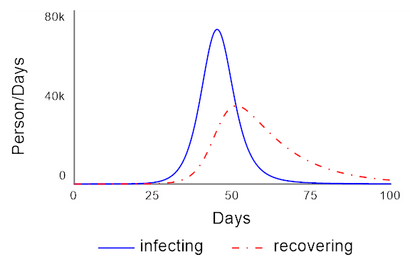
Most of the change is happening between days 25 and 60 or so. We can measure the overall "System Change" by weighting these flows by the total amount of change they cause over the course of the simulation. This value is displayed in the System Change tab on the Loops Panel:
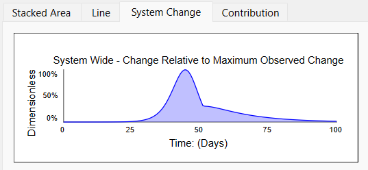
Then in the context of the System Change, it is possible to look at the contribution of each of the loops:
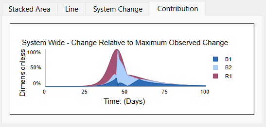
The contribution is the same as the Stacked Area graph will all loops selected but scaled to fit under the System Change curve. Here we see that the loops R1 and B2 are the most active loops during the period of significant change, while B1 remains active after the transition from growth to decline in infections.
The System Change and Contribution graphs thus allow you to focus in on specific loops during specific ranges of activity in the model.
Currently, models using DELAYN or SMTHN with a varaibles (instead of a number) as the order arguments will not work with Loops that Matter.
Also, models using discrete capabilities such as conveyors and the DELAY builtin use approximations for computing link scores as described in Discrete Variables and Special Equations.
Models using macros that inherently involve paths with different polarities (such as TREND and FORCST) are likely to yield ambiguous results. It is better, in these cases, to expand the macros into equations. The same is more generally true for macros (SMTH1, SMTH3, and so on) that form an important part of a feedback loop - expanding them will make the interactions much clearer as well as (usually) exposing a number of internal balancing feedback loops.